This is the second part of a series about designing metrics for event-driven systems. You can check the first part of this series.
Prometheus is open source system for monitoring and alerting. It is a part of CNCF (Cloud Native Computing Foundation) and it is one of the most popular monitoring systems. You can say it is a de facto standard for monitoring in Kubernetes.
To design metrics with Prometheus, you need to understand its metric types. In this article, I’ll explain Prometheus metric types and how to design metrics with them.
Prometheus Metric Types
All data in Prometheus is stored as time series. Time series is a set of data points indexed by time. The data point is a tuple of a timestamp and value. A time series is uniquely identified by its metric name and an optional set of key-value pairs called labels. Labels are used for Prometheus dimensional data model.
Prometheus has four metric types: Counter, Gauge, Histogram, and Summary.
Counter
For values that increase over time or can reset to zero on a restart, we use Counter. It is a cumulative metric that in essence is a monotonically increasing counter.
Some examples are the number of requests served, number of errors, number of bytes received, and so on. Use it for values that can only increase.
Gauge
If you have a single numerical value that can arbitrarily go up and down, you should use Gauge.
Some examples are temperature, current memory usage, current CPU usage, and so on. Use it for values that can increase and decrease.
Histogram
Histogram is a cumulative metric that represents the distribution of a set of values. It counts the number of observations in predefined buckets. As well, it provides a sum of all observed values.
Histogram named <basename> expose multiple metrics:
- counter for observed events: number of observations as Counter metric named
<basename>_count - total sum of observed values: sum of all observations as Counter metric named
<basename>_sum - cumulative counters for each bucket: number of observations per bucket as Counter metric named
<basename>_bucket{le="<upper inclusive bound>"}
Summary
Summary is a Histogram with the ability to calculate configurable quantiles over a sliding time window. It exposes:
- streaming f-quantiles (0 ≤ f ≤ 1) over a sliding time window as
<basename>{quantile="<f>"} - total sum: sum of all observations as Counter metric named
<basename>_sum - counter of all observed events: number of observations as Counter metric named
<basename>_count
There are subtle differences between Histogram and Summary. You can read more about them in Prometheus documentation.
In most cases, you would use Histogram.
Labels
As I already mentioned, labels are used for Prometheus dimensional data model. They are key-value pairs that are attached to a metric. Whenever some metric is observed, we attach labels to it. They carry additional information about observed metrics. Later we use them for grouping and filtering.
Important to remember is not to use labels for values that can change over time. That means that each label should have a finite number of possible values. That number should be small. Smaller the better. And try to keep the number of labels small. A large number of labels or a large number of label values can cause high cardinality. High cardinality is a problem because it can cause high memory usage and slow down Prometheus.
The RED Method and Prometheus Metric Types
Key metrics are:
- Request Rate
- Request Error rate
- Request Duration
Request Rate
Request rate metrics is a request rate per second. We can use a Counter for calculating the request rate. Counter as a cumulative metric will increase over time. Then we observe the rate of change of the Counter over time. Prometheus’s built-in function rate calculates the rate of increase of the time series in the last given period.
Say that a metric http_requests_total is a Counter. It counts the total number of HTTP requests. We calculate the request rate with:
sum(rate(http_requests_total[5m]))
Above you read as an average rate of change of http_requests_total in the last 5 minutes. In other words, it is the average number of requests per second in the last 5 minutes.
The sum function is used to aggregate the rate of change of all instances of the same service.
Request Error Rate
Let’s continue with http_requests_total metric. For each received request, we increase the http_requests_total Counter. As well we add a label status_code which
is the HTTP status code of the response. Now, whenever we increase http_requests_total Counter we’ll have information about the response status code. One more
time rate function will help us:
sum(rate(http_requests_total{status_code=~"5.."}[5m]))
We filter by status_code label, then we calculate the rate of change of the Counter over time. The expression reads as an average rate of errors per second
in the last 5 minutes.
The sum function is used to aggregate the rate of change of all instances of the same service.
Request Duration
For this metric, we need to use Histogram. Let’s name the metric http_request_duration_seconds, to express that it is in seconds. As well we need to define buckets:
0.005, 0.01, 0.025, 0.05, 0.1, 0.25, 0.5, 1, 2.5, 5, 10. This all means whenever we receive a request we measure its duration and we put it in the appropriate bucket.
Based on that we can calculate the average request duration. For that we use histogram_quantile function:
histogram_quantile(0.95, sum by (le) (rate(http_request_duration_seconds_bucket[5m])))
A quantile defines a particular part of the data set. In common words how many values are less or above a given value? In the expression above we are calculating 99th percentile. It will tell us the average duration of 95% of requests.
First, we calculate the rate of change of the Histogram over time and then sum all buckets. The histogram_quantile function will do the rest of the calculations. By
Prometheus definition http_request_duration_seconds_bucket is a counter.
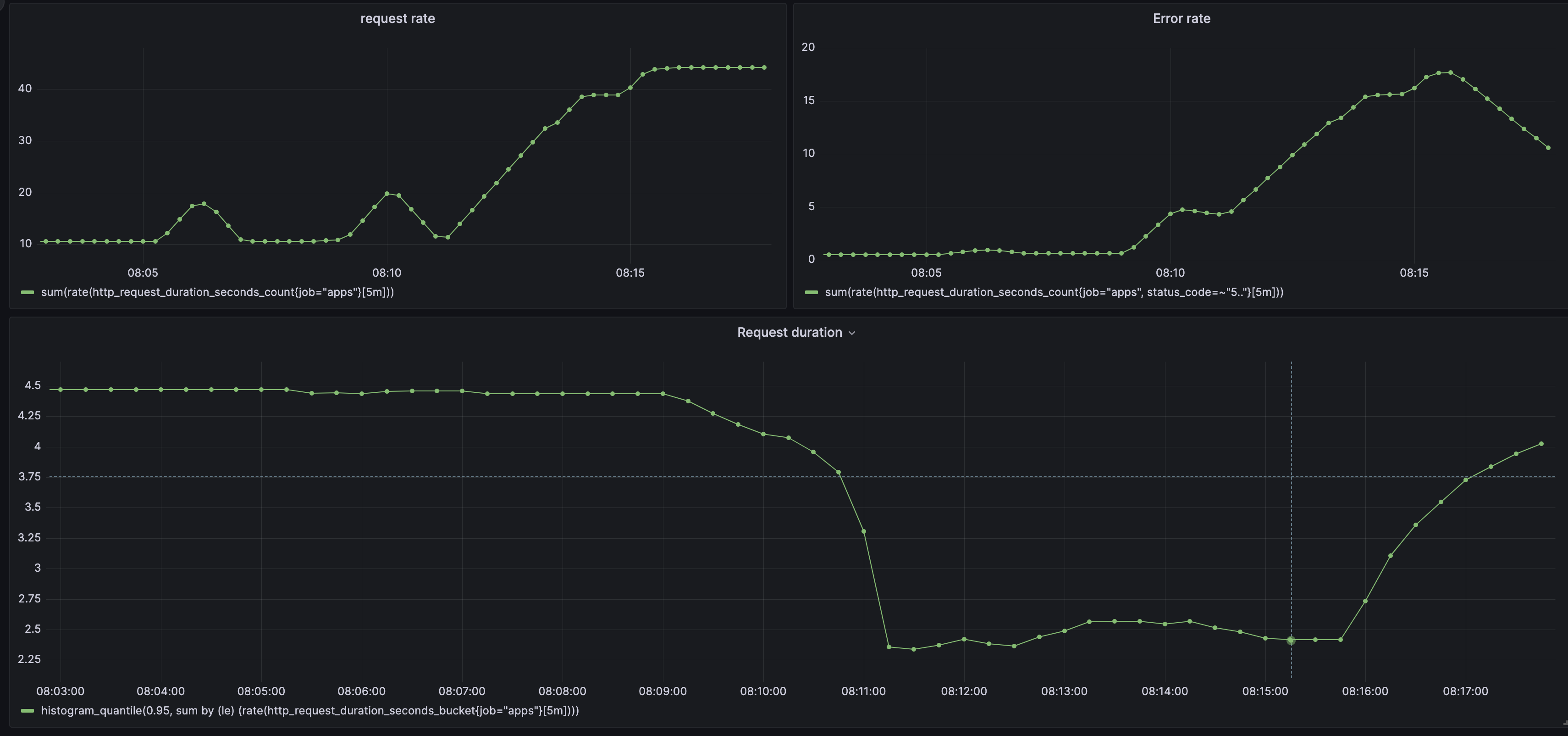
Redefined Request Rate and Error Rate
Since we are using Histogram for request duration, we can calculate the request rate and error rate with Histogram, too. Remember that one Histogram metric exposes
multiple counters: <name>_count, <name>_sum, and <name>_bucket. We can use <name>_count for the request rate. If we add the label status_code we can use it for the
error rate:
sum(rate(http_request_duration_seconds_count[5m])) ## request rate

sum(rate(http_request_duration_seconds_count{status_code=~"5.."}[5m])) ## error rate
So, we do not need to define a separate metric for the request rate and error rate since we can use Histogram for that.
Example
If you want to try Grafana and Prometheus you can checkout my docker compose playground. It contains Grafana, Prometheus, and a simple Go application that exposes.
Next
In the next part, I’ll try to explain the USE Method and how to use it with Prometheus. Any feedback is welcome. Thank you for reading.
If you would like to be notified when the next part is published, you can subscribe to my newsletter below.